library(tidyverse)
library(rgee)
library(tidyrgee)
library(sf)
library(stars)
library(viridis)
library(ggplot2)
library(mapview)
ee_Initialize()
#> ── rgee 1.1.5 ─────────────────────────────────────── earthengine-api 0.1.326 ──
#>  ✔ user: not_defined
#>  ✔ Initializing Google Earth Engine:
 ✔ Initializing Google Earth Engine:  DONE!
#>
 ✔ Earth Engine account: users/ambarja
#> ────────────────────────────────────────────────────────────────────────────────🔴 1. Exploratory Spatial Data Analysis
Before creating a spatial machine learning model, let’s explore some of the data sets available from Earth Engine using the rgee package within R. In this dataset there are climatic, environmental, vegetation and other variables that may be of interest.
1.1 Quickly review of Data catalog

1.2 Exploring dataset with rgee
The Earth Engine DataSet has several variables, in this example, we are going to visualize the elevation and ndvi dataset.
# Setup the colour palette with the elevation values
viz = list(
  min = 500,
  max = 5000,
  palette = rocket(n = 100,direction = -1)
  )
# Mapping the world elevation
ee$Image("CGIAR/SRTM90_V4") %>%
Map$addLayer(name = "Elevation",visParams = viz) +
Map$addLegend(visParams = viz, name = "Elevation")Exploring the MOD13Q1.061 dataset with tidyrgee and calculate the mean, sd, maximum and minimum NDVI and EVI value from 2000 to 2022.
modis_ic <- ee$ImageCollection$Dataset$MODIS_061_MOD13Q1 |>
as_tidyee()head(modis_ic$vrt)
#> # A tibble: 6 × 8
#> id time_start syste…¹ date month year doy band_…²
#> <chr> <dttm> <chr> <date> <dbl> <dbl> <dbl> <list>
#> 1 MODIS/061/MO… 2000-02-18 00:00:00 2000_0… 2000-02-18 2 2000 49 <chr>
#> 2 MODIS/061/MO… 2000-03-05 00:00:00 2000_0… 2000-03-05 3 2000 65 <chr>
#> 3 MODIS/061/MO… 2000-03-21 00:00:00 2000_0… 2000-03-21 3 2000 81 <chr>
#> 4 MODIS/061/MO… 2000-04-06 00:00:00 2000_0… 2000-04-06 4 2000 97 <chr>
#> 5 MODIS/061/MO… 2000-04-22 00:00:00 2000_0… 2000-04-22 4 2000 113 <chr>
#> 6 MODIS/061/MO… 2000-05-08 00:00:00 2000_0… 2000-05-08 5 2000 129 <chr>
#> # … with abbreviated variable names ¹system_index, ²band_namestidyrgee allows works with the tidyverse sintaxis, with this package you could use the functions of dplyr (s3 method) like filter, group_by and summarise.
# NDVI statistical using the group_by + summarise functions
modis_ndvi_yearly <- modis_ic |>
  select("NDVI") |>
  filter(date>="2016-01-01",date<="2019-12-31") |>
  group_by(year,month) |>
summarise(stat = "mean")head(modis_ndvi_yearly$vrt)
#> # A tibble: 6 × 8
#> year month dates…¹ numbe…² time_start time_end date
#> <dbl> <dbl> <list> <int> <dttm> <dttm> <date>
#> 1 2016 1 <dttm> 2 2016-01-01 00:00:00 2016-01-01 00:00:00 2016-01-01
#> 2 2016 2 <dttm> 2 2016-02-02 00:00:00 2016-02-02 00:00:00 2016-02-02
#> 3 2016 3 <dttm> 2 2016-03-05 00:00:00 2016-03-05 00:00:00 2016-03-05
#> 4 2016 4 <dttm> 2 2016-04-06 00:00:00 2016-04-06 00:00:00 2016-04-06
#> 5 2016 5 <dttm> 2 2016-05-08 00:00:00 2016-05-08 00:00:00 2016-05-08
#> 6 2016 6 <dttm> 2 2016-06-09 00:00:00 2016-06-09 00:00:00 2016-06-09
#> # … with 1 more variable: band_names <list>, and abbreviated variable names
#> # ¹dates_summarised, ²number_images1.3 Creating a set of variables for predicting malaria focus
Malaria is a disease that has a high recurrence in tropical places, this has multiple factors that condition its outbreak, including environmental and climatic factors has a high degree of significance, for this reason we will create a set of data to help predict their probability of occurrence using machine learning in the department of Loreto - Peru.
This malaria dataset 🦟 reported is from 2018, click here to download.
Variables to consider:
Temperature 🌡️
Precipitation 🌧️
NDVI 🍂
Exploring spatial dataset of Malaria 🦟
malaria_db <- st_read("dataset/malariadb2018.gpkg",quiet = T)
head(malaria_db)[1:4]
#> Simple feature collection with 6 features and 4 fields
#> Geometry type: POINT
#> Dimension:     XY
#> Bounding box:  xmin: -76.12383 ymin: -5.765671 xmax: -76.12383 ymax: -5.765671
#> Geodetic CRS:  WGS 84
#>       id_loc id2 nrohab      village                        geom
#> 1 1602010021   1    186 SANTA ISABEL POINT (-76.12383 -5.765671)
#> 2 1602010021   1    186 SANTA ISABEL POINT (-76.12383 -5.765671)
#> 3 1602010021   1    186 SANTA ISABEL POINT (-76.12383 -5.765671)
#> 4 1602010021   1    186 SANTA ISABEL POINT (-76.12383 -5.765671)
#> 5 1602010021   1    186 SANTA ISABEL POINT (-76.12383 -5.765671)
#> 6 1602010021   1    186 SANTA ISABEL POINT (-76.12383 -5.765671)
# P. falciparum cases by province
malaria_db |>
group_by(province) |>
summarise(fal = sum(fal,na.rm = T)) |>
ggplot(aes(x = reorder(province,fal),y = fal)) +
geom_bar(stat = "identity",fill = "blue",alpha = 0.6) +
coord_flip() + theme_minimal() +
labs(title = "P.Falciparum cases", x = "",y = "")
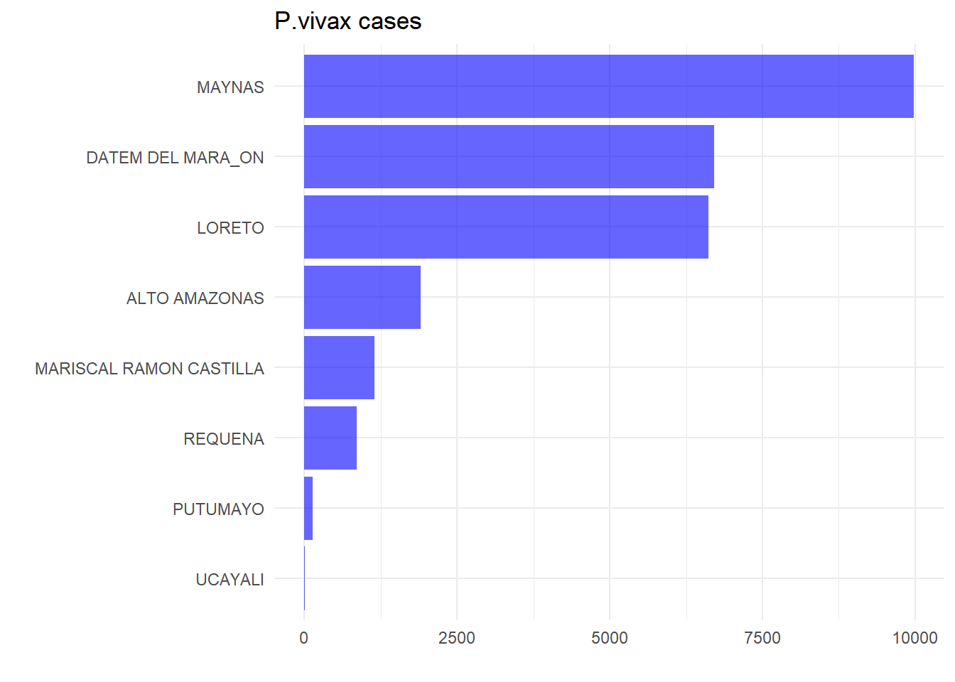
# P. vivax cases by province
malaria_db |>
group_by(province) |>
summarise(viv = sum(viv,na.rm = T)) |>
ggplot(aes(x = reorder(province,viv),y = viv)) +
geom_bar(stat = "identity",fill = "blue",alpha = 0.6) +
coord_flip() + theme_minimal() +
labs(title = "P.vivax cases", x = "",y = "")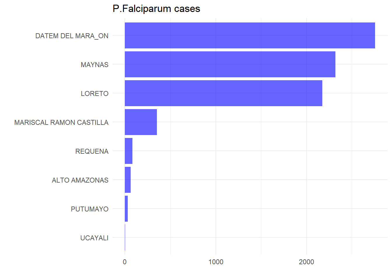
Mapping the total cases of P. falciparum and P.vivax
# Total cumulative cases per year
malaria_total <- malaria_db |>
  group_by(village) |>
  summarise(
    fal = sum(fal,na.rm = T),
    viv = sum(viv,na.rm = T)
    )
# Mapping P.falciparum
m1 <- malaria_total |>
mapview(
zcol = "fal",
cex = "fal",
lwd = 0.01,
layer.name = "P.falciparum")
#Mapping P.vivax
m2 <- malaria_total |>
mapview(
zcol = "viv",
cex = "viv",
lwd = 0.01,
layer.name = "P.vivax")
m1|m2
#> Loading required namespace: leaflet.extras2Pre-processing of selected variables (precipitation, temperature, NDVI and EVI) to create a complete dataset for modelling.
# Study area
loreto <- st_read("https://github.com/healthinnovation/sdb-gpkg/raw/main/box_loreto.gpkg")|>
  sf_as_ee()
#> Reading layer `box_loreto' from data source
#>   `https://github.com/healthinnovation/sdb-gpkg/raw/main/box_loreto.gpkg'
#>   using driver `GPKG'
#> Simple feature collection with 1 feature and 83 fields
#> Geometry type: MULTIPOLYGON
#> Dimension:     XY
#> Bounding box:  xmin: -77.83596 ymin: -8.725191 xmax: -69.93904 ymax: -0.02860597
#> Geodetic CRS:  WGS 84
#> Registered S3 method overwritten by 'geojsonsf':
#>   method        from
#>   print.geojson geojson
# Climate variables
terraclim_ic <- ee$ImageCollection$
Dataset$IDAHO_EPSCOR_TERRACLIMATE |>
as_tidyee()
# Vegetation variables
modis_ic <- ee$ImageCollection$
Dataset$MODIS_061_MOD13Q1 |>
as_tidyee()# Precipitation dataset
db_pp <- terraclim_ic |>
select("pr") |>
filter(year == "2018") |>
group_by(year,month) |>
summarise(stat= "sum")
# Temperature dataset
db_temp <- terraclim_ic |>
select("tmmx") |>
filter(year == "2018") |>
group_by(year,month) |>
summarise(stat= "mean")
# Vegetation index
db_ndvi <- modis_ic |>
select("NDVI") |>
filter(year == "2018") |>
group_by(year,month) |>
summarise(stat= "mean")# Precipitation legend
viz_pp <- list(
min = 462,
max = 8272,
palette = mako(n = 10,direction = -1)
)
# Temperature legend
viz_temp <- list(
min = 9.78,
max = 32.67,
palette = rocket(n = 10)
)
# NDVI lenged
viz_ndvi <- list(
min =0.35,
max = 0.79,
palette = viridis(n = 10)
)
Map$centerObject(loreto)
#> NOTE: Center obtained from the first element.# Precipitation mapping
m1 <- Map$addLayer(db_pp$ee_ob$sum()$clip(loreto),visParams = viz_pp) +
Map$addLegend(visParams = viz_pp, "Precipitation",position = "bottomleft")
# Temperature mapping
m2 <- Map$addLayer(db_temp$ee_ob$mean()$multiply(0.1)$clip(loreto),visParams = viz_temp) +
Map$addLegend(visParams = viz_temp,name = "Temperature", position = "bottomright")
m1 | m2# NDVI mapping
m3 <- Map$addLayer(
db_ndvi$ee_ob$mean()$multiply(0.0001)$clip(loreto),
visParams = viz_ndvi) +
Map$addLegend(visParams = viz_ndvi,name = "NDVI")
m3# Downloading ic to raster
ee_to_pp <- ee_as_raster(
image = db_pp$ee_ob$sum()$clip(loreto)$toDouble(),
region = loreto$geometry(),
scale = 1000,
dsn = "dataset/percipitation.tif")
ee_to_temp <- ee_as_raster(
image = db_temp$ee_ob$mean()$multiply(0.1)$clip(loreto)$toDouble(),
region = loreto$geometry(),
scale = 1000,
dsn = "dataset/temperature.tif")
ee_to_ndvi <- ee_as_raster(
image = db_ndvi$ee_ob$mean()$multiply(0.0001)$clip(loreto)$toDouble(),
region = loreto$geometry(),
scale = 1000,
dsn = "dataset/ndvi.tif")# Creating a dataset for modeling
malaria_annual <- malaria_db %>%
group_by(village) %>%
summarise(fal = sum(fal,na.rm = TRUE)) %>%
st_cast("POINT")# Reading the variables stack
stack_variables <- list.files(
"dataset/",
pattern ="*.tif$"
) %>%
sprintf("dataset/%s",.) %>%
raster::stack()
names(stack_variables) <- c("ndvi","pp","temp")# Dataset for model
db_for_model <- st_extract(
st_as_stars(stack_variables),
malaria_annual) %>%
st_as_sf() %>%
mutate(
malaria = malaria_annual$fal,
lat = st_coordinates(.)[,2],
lon = st_coordinates(.)[,1]
) %>%
st_set_geometry(NULL)
names(db_for_model) <- c("ndvi","pp","temp","malaria","lat","lon")🔴 2. Random Forest Model
fit = glm(malaria ~ pp + temp + ndvi,
          family = poisson(),
          data = db_for_model)
🔴 3. Predicition Malaria
# making the prediction
pred = terra::predict(stack_variables, model = fit, type = "response")